Marginal Likelihood
Note: This is my blog’s first post but the presented function was not the first coded function for this package. In fact there has been almost been half a year now since I started developing this package.
Summary
In this post I will show you how the marginal_likelihood function was derived by the code presented by Merkle et al. (2019) for usage with models fitted with the birtms package. The code’s performance has been improved and the range of item response theory (IRT) models it can be calculated for has been increased. Since a birtmsfit object is an extension of a brmsfit object you can use the code presented here for many latent variable models fitted with brms (Bürkner, 2020b) after some slight adjustments.
Glance of theory
Comparing models
When I came along the article comparing conditional and marginal likelihoods for latent variable models by Merkle et al. (2019) at the end of 2020 I already fit a bunch of IRT models with brms. And I used the Pareto-smoothed importance sampling (PSIS) leave-one-out cross validation criteria (LOO-CV) (Vehtari et al., 2017) to compare the model fit among those although I was aware that this criteria might lead to wrong decisions.
How does LOO-CV work? In LOO-CV we remove a single response (or more precise: a single row of our long-format data set) and fit our model of interest. After that we check how good our model predicts the removed response. We repeat this for every response and end up with an estimation of how good our full model predicts new responses. Because fitting a model in a Bayesian takes considerably more time than with non-Bayesian methods fitting such a model again and again and again would take a huge amount of time.
Let’s look at two examples: If you fit a three parametric testlet model (Wainer et al., 2007) with around 100 persons with 270 responses each this might take three days - for a single run. To calculate the expected log pointwise predictive density (elpd) via exact LOO-CV you would have to fit this model 27.000 times. It would take round about 222 years! Fitting the (way simpler) Rasch model to the same data still takes 20 minutes for a single run - thus resulting in a computation time of one xear for the exact loo elpd. No can do that.
Fortunately Vehtari et al. (2017) found a way to efficiantly estimate the loo elpd via Paretho-smoothing using the posterior samples of our Bayesian models. This way we get a robust estimate of the loo elpd at the cost of some minutes computation time in most cases. I was willing to spend this amount of time to get the state-of-the-art estimate for models’ predictive error - which is superior to AIC, DIC and even WAIC (Vehtari et al., 2017). One super cool feature of PSIS LOO-CV is: it gives you a parameter (called Pareto k) that warns you if your model is to flexible1.
But of course this method has some limitations as well. And one of them strikes us when we fit latent variable (or hierarchical) models: With LOO-CV we remove just a single response at a time. But these responses aren’t independent from eachother because they all are related to one person (or cluster). Thus we might get an overoptimistic elpd value because it should be easier to predict a response based on the other responses a person gave compared to predict it by the other persons responses. So we would have to remove all the answers of a person at a time to get an unbiased estimate. Vehtari et al. (2017) state that - in theory - it is possible to do importance-sampling in this cases - but the more responses are related to a single person the more likely this method will result in a bad elpd estimate. Therefore they recommend using k-fold cross validation instead of LOO-CV in these cases, because this it is possible to partition the data accounting for the hierarchical structure (Vehtari, 16.12.2020).
Let’s see if k-fold cross validation is a method we could use instead of PSIS LOO-CV in daily work. If we remove all the responses of \(\frac{1}{10}\)th of the persons in our dataset, fit the model and calculate the predictive error and repeat this 10 times we get a robust estimate for the elpd. This will take about three hours for our Rasch model and a month for the 3pl testlet model. The former can be done over night - the latter not. And if we don’t remove \(\frac{1}{10}\)th of the persons (and their responses) but only one persons responses at a time we have to fit the model as many times as persons contributed responses to our dataset. Therefore this will take even longer. Maybe we just should stick to the simpler models? Or being more patient? Or get better hardware? Or just use PSIS LOO-CV as long as it does not yield high Pareto k’s?
I first decided to just use the PSIS LOO-CV criteria and hope that the worse elpd estimates won’t lead to wrong decisions at model comparison. I mean - Bürkner (2020a) did so in his awesome vignette and in their case study Vehtari (16.12.2020) found that the order of the models was preserved and only the elpd differences varied. But some weeks ago I found the article by Merkle et al. (2019) who tackle exactly this issue. Therefore I decided to work through the difference between conditional and marginal likelihoods and implement their approach for the birtms package.
Note: Right now I have no case study results to present here comparing the decisions I would have made based on PSIS LOO-CV criteria using conditional vs marginal likelihood. But I will write another blog post on this question later.
The likelihood type matters
Merkle et al. (2019) discuss the importance of the marginal likelihood for information criteria computation of latent variable models. They contrast the marginal likelihood with the conditional likelihood and argue: one should use the marginal likelihood if it’s of interest how well the model predicts the responses of a new person. Only if it’s of interest how well the model predicts additional responses of an already present person one should use the conditional likelihood. Thus in psychometric contexts we should use the marginal likelihood most of the time2.
One important information for me was: they don’t talk about the marginal likelihood as used for Bayes factor (BF) computation (which might come to your mind first if you worked in Bayesian modeling for some time). They talk about the marginal likelihood as it is commonly used in (frequentist) IRT modeling. Further their conditional likelihood is called joint maximum likelihood elsewhere. I think all these terms are pretty confusing. So let’s have a short look at the corresponding likelihoods’ (L) formulas in the context of a dicotomous Rasch model3 to understand the difference:
\[ \begin{align} & \mathrm{L} & = & \prod_{i,j}{p\left( y_{ij} | \phi \right)} \\ & \mathrm{L}_{conditional} & = & \prod_{i,j}{p\left( y_{ij} | \beta_i, \theta_j \right)} \\ & \mathrm{L}_{marginal} & = & \prod_{i,j}{p\left( y_{ij} | \beta_i, \psi \right)} \\ & & & p\left( y_{ij} | \beta_i, \psi \right) = \int_{\theta_j}{p\left( y_{ij} | \beta_i, \theta_j\right)p\left( \theta_j | \psi\right) \mathrm{d}\theta_j} \\ & \mathrm{L}_{BF} & = & \prod_{i,j}{p\left( y_{ij} | \alpha \right)}\\ & & & p\left( y_{ij} | \rho \right) = \int_\phi{p\left( y_{ij} | \phi\right)p\left( \phi | \rho\right) \mathrm{d}\phi} \end{align} \]
Here \(\phi\) represents a set of all model parameters - for a Rasch model these are the item locations4 \(\beta_i\) and the person locations5 \(\theta_j\). In many approaches the item parameters are considered as fixed effects and the person parameters are random effects with a specific prior distribution (e. g. \(\theta \sim N(0, 1)\)) and the person parameters are not of direct interest (Merkle et al., 2019). Therefore the specific values get substituted by their distribution in the likelihood.
However, following the tutorial on IRT modeling with brms (Bürkner, 2020a) I handle the item parameters as random effects as well to benefit from the partial pooling effect. We will get estimates for item and person parameters anyway. But we won’t substitute the item parameters specific values with their distribution6.
The argumentation to use marginal likelihood in most psychometric contexts because we generally want to predict responses from a new person seems pretty convincing to me. But do we find beneficial properties of information criteria derived from the marginal likelihood as well? Yes, indeed. Merkle et al. (2019) showed that the Monte Carlo error for information criteria based on the marginal likelihood is much lower7. A precision gain is nice.
But what really seems to be an issue is the following: The order in model fit ranking can be different comparing information criteria derived from conditional and marginal likelihood. E.g.: Merkle et al. (2019) assume that conditional DIC generally prefers more more complex models as marginal DIC. Further they found that DIC and WAIC better approximate PSIS-LOO for marginal information criteria - thus being more consistent. Last but not least: they “expect similar issues to arise when one uses posterior predictive estimates to study model fit” (Merkle et al., 2019).
This brings me back to my own former conclusions. In model comparison via PSIS-LOO I found that a 3PL testlet model with a common guessing parameter (hence almost a 2PL testlet model) suits the data best. But I simply used the default functions for log likelihood calculation. And the default likelihood is the conditional one! Thus I will do the model selection process once again once I coded a suitable function for multidimensional IRT models8.
Be aware: Using the brms package to fit models you find a function called brms::log_lik(). This function will calculate the pointwise log-likelihood. Thus it is calculated by taking the logarithm of the conditional likelihood. Therefore the brms::waic() and brms::loo() functions will result in information criteria based on the conditional likelihood9. This does not suit the recommandations of Merkle et al. (2019).
So what to do? Do you have to work through all the formula in the articles of Merkle et al. (2019) and Rabe-Hesketh et al. (2005) to understand the algorithm and code a function all by yourself? No you don’t. And I didn’t either. Just keep reading and see how a suitable function was prepared for you.
Calculating the marginal likelihood
Fortunately, along with their article Merkle et al. (2019) published the R code of their calculations in the online supplementary material. They use the edstan package (Furr, 2017) to fit a Rasch model with some custom Stan code in the generated quantities block to get the latent person ability scores10.
The edstan package somes with some Stan code presets for IRT models. But personally I found it a bit cumbersome to alter the Stan code by hand to fit the model in my mind and therefore prefer formulating my model as a generalised (nonlinear) regression model and let brms generate the Stan code for me11. In the remaining blog post I want to show you the adjustments and extensions I made to their code to calculate the marginal likelihood with birtmsfit objects and hope you can adapt it yourself to work on brmsfit objects of latent variable models more generally.
First I will show you the original code by Merkle et al. (2019):
# Function to obtain marginal likelihoods with parallel processing.
# stan_fit: Fitted Stan model
# data_list: Data list used in fitting model
# MFUN: Function to calculate marginal likelihood for cluster at a node
#   location. This is application specific.
# resid_name: Name of residual in Stan program to integrate out
# sd_name: Name of SD for residual in Stan program
# n_nodes: Number of adaptive quadrature nodes to use
# best_only: Whether to evaluate marginal likelihood only at posterior means
mll_parallel <- function(stan_fit, data_list, MFUN, resid_name, sd_name, n_nodes,
                         best_only = FALSE) {

  library(foreach)
  library(statmod)       # For gauss.quad.prob()
  library(matrixStats)   # For logSumExp()

  draws <- rstan::extract(stan_fit, stan_fit@model_pars)
  n_iter <- ifelse(best_only, 0, nrow(draws$lp__))
  post_means <- better_posterior_means(stan_fit)

  # Seperate out draws for residuals and their SD
  resid <- apply(draws[[resid_name]], 2, mean)
  stddev <- apply(draws[[resid_name]], 2, sd)

  # Get standard quadrature points
  std_quad <- gauss.quad.prob(n_nodes, "normal", mu = 0, sigma = 1)
  std_log_weights <- log(std_quad$weights)

  # Extra iteration is to evaluate marginal log-likelihood at parameter means.
  ll <- foreach(i = 1:(n_iter + 1), .combine = rbind,
                .packages = "matrixStats") %dopar% {

    ll_j <- matrix(NA, nrow = 1, ncol = ncol(draws[[resid_name]]))

    for(j in 1:ncol(ll_j)) {

      # Set up adaptive quadrature using SD for residuals either from draws or
      # posterior mean (for best_ll).
      sd_i <- ifelse(i <= n_iter, draws[[sd_name]][i], post_means[[sd_name]])
      adapt_nodes <- resid[j] + stddev[j] * std_quad$nodes
      log_weights <- log(sqrt(2*pi)) + log(stddev[j]) + std_quad$nodes^2/2 +
        dnorm(adapt_nodes, sd = sd_i, log = TRUE) + std_log_weights

      # Evaluate mll with adaptive quadrature. If at n_iter + 1, evaluate
      # marginal likelihood at posterior means.
      if(i <= n_iter) {
        loglik_by_node <- sapply(adapt_nodes, FUN = MFUN, r = j, iter = i,
                                 data_list = data_list, draws = draws)
        weighted_loglik_by_node <- loglik_by_node + log_weights
        ll_j[1,j] <- logSumExp(weighted_loglik_by_node)
      } else {
        loglik_by_node <- sapply(adapt_nodes, FUN = MFUN, r = j, iter = 1,
                                 data_list = data_list, draws = post_means)
        weighted_loglik_by_node <- loglik_by_node + log_weights
        ll_j[1,j] <- logSumExp(weighted_loglik_by_node)
      }

    }

    ll_j

  }

  if(best_only) {
    return(ll[nrow(ll), ])
  } else {
    return(list(ll = ll[-nrow(ll), ], best_ll = ll[nrow(ll), ]))
  }

}


# Function to calculate likelihood for a cluster for an adaptive quad node
# specific to the IRT example. Similar functions would be written for other
# applications and passed to mll_parallel().
# node: node location
# r: index for cluster
# iter: mcmc iteration
# data_list: data used to fit Stan model
# draws: mcmc draws from fitted Stan model
f_marginal <- function(node, r, iter, data_list, draws) {
  y <- data_list$y[data_list$jj == r]
  theta_fix <- draws$theta_fix[iter, r]
  delta <- draws$delta[iter, data_list$ii[data_list$jj == r]]
  p <- boot::inv.logit(theta_fix + node - delta)
  sum(dbinom(y, 1, p, log = TRUE))
}
General remarks: The function mll_parallel uses parallel processing to speed up the calculation. That’s sweet. I didn’t knew about foreach package (Microsoft & Weston, 2020) before and was happy to learn some new tricks I might use in my upcoming package as well. On my machine the calculation of the marginal likelihood for the examplary unidimensional Rasch model takes about 158 seconds12. But what we definetly don’t want are the library() calls inside of the function (just to get one or two functions of the packages). Instead we will work with the :: operator13, e.g. matrixStats::logSumExp().
In the next code block we will follow Merkle et al. (2019) fitting the IRT model on the verbal aggression dataset with the edstan package and a customized Stan script. Next we calculate the marginal likelihood using the code above and finish with printing the LOO-CV statistics and a nice Pareto k plot. These will be used as reference for the functions coded for the use with birtms objects following beneath.
library(rstan)
library(doParallel)
library(loo)
library(tidyverse)
options(mc.cores = 4)
options(loo.cores = 4)

aggression <- edstan::aggression

# Assemble example dataset; the considered model formula is
#   ~ 1 + male + anger;
dl <- edstan::irt_data(y = aggression$dich, jj = aggression$person,
               ii = aggression$item, covariates = aggression,
               formula = ~ 1 + male + anger)

# Fit model (or load fitted model)
if (!file.exists('data/stan_fit.rds')) {
  stan_fit <- rstan::stan("data/rasch_edstan_modified.stan", data = dl, iter = 2000, chains = 4) # we draw more samples with one chain less
  saveRDS(stan_fit, file = 'data/stan_fit.rds')

  cl <- makeCluster(4)
  registerDoParallel(cl)
  ll_marg <- mll_parallel(stan_fit, dl, f_marginal, "zeta", "sigma", 11)
  stopCluster(cl)
  saveRDS(ll_marg, file = 'data/ll_marg.rds')
} else {
  stan_fit <- readRDS('data/stan_fit.rds')

  ll_marg <- readRDS('data/ll_marg.rds')
}

chain <- stan_fit %>% tidybayes::spread_draws(sigma) %>% pull(.chain)
loo_ll_marg <- loo(ll_marg$ll, r_eff = relative_eff(ll_marg$ll, chain))

print(loo_ll_marg)
##
## Computed from 4000 by 316 log-likelihood matrix
##
##          Estimate    SE
## elpd_loo  -4057.4  64.4
## p_loo        27.6   0.6
## looic      8114.7 128.8
## ------
## Monte Carlo SE of elpd_loo is 0.1.
##
## All Pareto k estimates are good (k < 0.5).
## See help('pareto-k-diagnostic') for details.
plot(loo_ll_marg)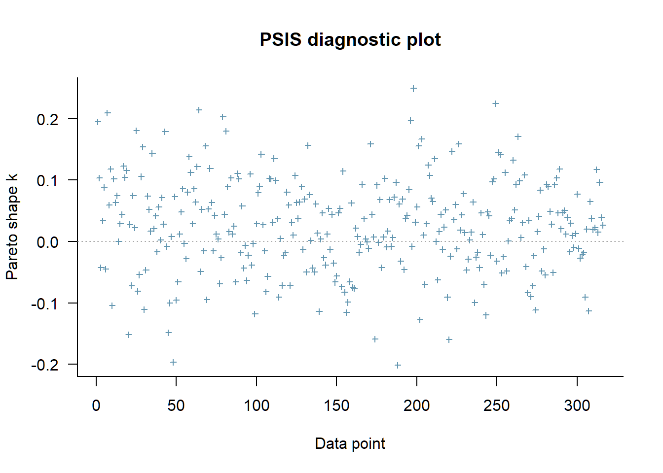
As we can see the likelihood was evaluated at around 300 points. These are related to the 316 persons who answered 24 items each. We find no Pareto k over .5. Actually we find some with negative value, which is fine. We should be concerned if we find values over .7. In the next section we will fit the model above twice with brms.
Conditional likelihood with brms
First we fit the model with items as fixed effects which equals the model we fitted with edstan before. Second we fit the model with items as random effects which follows Bürkner (2020a) recommondations and will be equal to the models fit with birtms.
library(brms)
## Loading required package: Rcpp
## Loading 'brms' package (version 2.14.4). Useful instructions
## can be found by typing help('brms'). A more detailed introduction
## to the package is available through vignette('brms_overview').
##
## Attaching package: 'brms'
## The following object is masked from 'package:rstan':
##
##     loo
## The following object is masked from 'package:stats':
##
##     ar

aggression <- aggression %>% mutate(item = as.character(item))

formula_aggression_1pl_fixed <- bf(dich ~ 1 + item + (1 | person) + male + anger)
formula_aggression_1pl_random <- bf(dich ~ 1 + (1 | item) + (1 | person) + male + anger)

# Fit model (or load fitted model)
if (!file.exists('data/fit_aggression_1pl_fixed.rds')) {
  fit_aggression_1pl_fixed <- brm(
    formula = formula_aggression_1pl_fixed,
    data = aggression,
    family = brmsfamily("bernoulli", "logit"),
    file = 'data/fit_aggression_1pl_fixed.rds'
  )
  fit_aggression_1pl_fixed <- add_criterion(fit_aggression_1pl_fixed, 'loo') # does not save automatically for some reason
  saveRDS(fit_aggression_1pl_fixed, file = 'data/fit_aggression_1pl_fixed.rds')

  # ll_cond_fixed <- log_lik(fit_aggression_1pl_fixed)
  # saveRDS(ll_cond_fixed, file = 'data/ll_cond_fixed.rds')
} else {
  fit_aggression_1pl_fixed <- readRDS('data/fit_aggression_1pl_fixed.rds')

  # ll_cond_fixed <- readRDS('data/fit_aggression_1pl_fixed.rds')
}

if (!file.exists('data/fit_aggression_1pl_random.rds')) {
  fit_aggression_1pl_random <- brm(
    formula = formula_aggression_1pl_random,
    data = aggression,
    family = brmsfamily("bernoulli", "logit"),
    file = 'data/fit_aggression_1pl_random.rds'
  )
  fit_aggression_1pl_random <- add_criterion(fit_aggression_1pl_random, 'loo')

  # ll_cond_random <- log_lik(fit_aggression_1pl_random)
  # saveRDS(ll_cond_random, file = 'data/ll_cond_random.rds')
} else {
  fit_aggression_1pl_random <- readRDS('data/fit_aggression_1pl_random.rds')

  # ll_cond_random <- readRDS('data/fit_aggression_1pl_random.rds')
}

loo(fit_aggression_1pl_fixed, fit_aggression_1pl_random)
## Output of model 'fit_aggression_1pl_fixed':
##
## Computed from 4000 by 7584 log-likelihood matrix
##
##          Estimate   SE
## elpd_loo  -3868.4 44.3
## p_loo       290.7  4.2
## looic      7736.8 88.6
## ------
## Monte Carlo SE of elpd_loo is 0.2.
##
## All Pareto k estimates are good (k < 0.5).
## See help('pareto-k-diagnostic') for details.
##
## Output of model 'fit_aggression_1pl_random':
##
## Computed from 4000 by 7584 log-likelihood matrix
##
##          Estimate   SE
## elpd_loo  -3868.0 43.8
## p_loo       288.1  4.1
## looic      7736.1 87.5
## ------
## Monte Carlo SE of elpd_loo is 0.2.
##
## All Pareto k estimates are good (k < 0.5).
## See help('pareto-k-diagnostic') for details.
##
## Model comparisons:
##                           elpd_diff se_diff
## fit_aggression_1pl_random  0.0       0.0
## fit_aggression_1pl_fixed  -0.4       0.8
plot(loo(fit_aggression_1pl_fixed))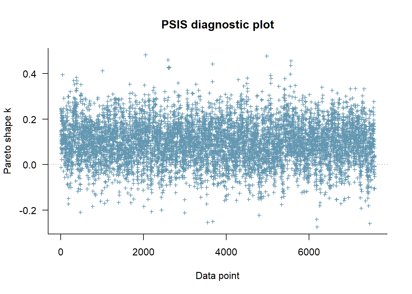
As we see both approaches fit just as well and it took 19 s to compute each of the conditional likelihoods - instead of 158 s. Compared to the marginal loo we see that their elpd_loo is almost 200 lower - we migth tend to interpret this as: the brms models have better fitting. But we musn’t compare the elpd by their value because the likelihoods types differ and have different length. Since the models are basicly the same we should wonder about this big elpd difference. My interpretation right now is: this might be linked to the finding in Merkle et al. (2019) that conditional likelihoods tend to support more complex models - but I’m not sure. Looking at the plot we see again that the conditional information criteria is based on the individual responses and not clustered by person resulting in many more blue crosses.
Marginal likelihood with brms
MFUN0 <- function(node, r, iter, data_list2, draws2, linear_terms) {
  resp_numbers <- data_list2[data_list2$person == unique(data_list2$person)[[r]],"resp_number"]

  y <- data_list2$dich[resp_numbers]
  base_term <- linear_terms[iter, resp_numbers] - draws2$theta[[iter, r]]

  p <- brms::inv_logit_scaled(base_term + node)
  sum(dbinom(y, 1, p, log = TRUE))
}

mll_parallel_brms1 <- function(fit, MFUN, n_nodes = 11, best_only = FALSE, cores = 4) {

  # ----- create a temporary logging file ----
  tempDir <- tempfile()
  dir.create(tempDir)
  logFile <- file.path(tempDir, "log.txt")
  viewer <- getOption("viewer")
  viewer(logFile)

  # ----- initialise multiple workers ----
  cl <- parallel::makeCluster(cores, outfile = logFile)
  doParallel::registerDoParallel(cl)
  on.exit(parallel::stopCluster(cl)) # terminate workes when finished

  # we get the dataset from the brms fit and add row and person numbers instead of passing it to the function
  data_list2 <- fit$data %>% mutate(resp_number = row_number(),
                                    person_number = as.numeric(factor(person, levels = unique(person))))

  #browser()

  draws2 <- list(sd = tidybayes::spread_draws(fit, sd_person__Intercept) %>%
                   rename(sd_person = sd_person__Intercept) %>%
                   select(!starts_with('.')),
                 theta = tidybayes::spread_draws(fit, r_person[person,]) %>%
                   pivot_wider(values_from = r_person, names_from = person) %>%
                   select(!starts_with('.'))
                 )

  n_iter2 <- nsamples(fit)

  post_means2 <- map(draws2, ~matrix(colMeans(.), nrow = 1))

  # Seperate out draws for residuals and their SD
  resid2 <- ranef(fit)$person[,1,1]
  stddev2 <- ranef(fit)$person[,2,1]

  n_persons <- length(resid2)

  # Get standard quadrature points
  std_quad <- statmod::gauss.quad.prob(n_nodes, "normal", mu = 0, sigma = 1)
  std_log_weights <- log(std_quad$weights)

  linear_terms <- fitted(fit, scale = 'linear', summary = FALSE)
  linear_terms_mean <- matrix(colMeans(linear_terms), nrow = 1)

  # Extra iteration is to evaluate marginal log-likelihood at parameter means.
  ll <- foreach::`%dopar%`(foreach::foreach(i = 1:(n_iter2 + 1), .combine = rbind,
                                            .packages = "matrixStats"
                                            ),
                           {
                  my_options <- options(digits.secs = 3)
                  on.exit(options(my_options))

                  if(i %% 100 == 0 ) {
                    print(paste(i, strptime(Sys.time(), "%Y-%m-%d %H:%M:%OS") ))
                  }

                  ll_j <- matrix(NA, nrow = 1, ncol = n_persons)

                  for(j in 1:n_persons) {

                    # Set up adaptive quadrature using SD for residuals either from draws or
                    # posterior mean (for best_ll).
                    sd_i <- ifelse(i <= n_iter2, draws2$sd$sd_person[[i]], post_means2$sd[[1]])
                    adapt_nodes <- resid2[[j]] + stddev2[[j]] * std_quad$nodes
                    log_weights <- log(sqrt(2*pi)) + log(stddev2[[j]]) + std_quad$nodes^2/2 +
                      dnorm(adapt_nodes, sd = sd_i, log = TRUE) + std_log_weights

                    # Evaluate mll with adaptive quadrature. If at n_iter + 1, evaluate
                    # marginal likelihood at posterior means.
                    if(i <= n_iter2) {

                      loglik_by_node <- sapply(adapt_nodes, FUN = MFUN, r = j, iter = i,
                                               data_list = data_list2, draws = draws2, linear_terms = linear_terms)

                      weighted_loglik_by_node <- loglik_by_node + log_weights
                      ll_j[1,j] <- matrixStats::logSumExp(weighted_loglik_by_node)
                    } else {
                      loglik_by_node <- sapply(adapt_nodes, FUN = MFUN, r = j, iter = 1,
                                 data_list = data_list2, draws = post_means2, linear_terms = linear_terms_mean)

                      weighted_loglik_by_node <- loglik_by_node + log_weights
                      ll_j[1,j] <- matrixStats::logSumExp(weighted_loglik_by_node)
                    }

                  }

                  ll_j

                })

  if(best_only) {
    return(ll[nrow(ll), ])
  } else {
    return(list(ll = ll[-nrow(ll), ], best_ll = ll[nrow(ll), ]))
  }

}

MFUN1 <- function(node, r, iter, data_list2, draws2, linear_terms) {
  resp_numbers <- data_list2$resp_number[data_list2$person_number == r]
  y <- data_list2$dich[resp_numbers]
  base_term <- linear_terms[iter, resp_numbers] - draws2$theta[[iter, r]]

  p <- brms::inv_logit_scaled(base_term + node)
  sum(dbinom(y, 1, p, log = TRUE))
}

# uses matrix objects instead of tibbles to store data
mll_parallel_brms2 <- function(fit, MFUN, n_nodes = 11, best_only = FALSE, cores = 4) {

  # ----- create a temporary logging file ----
  tempDir <- tempfile()
  dir.create(tempDir)
  logFile <- file.path(tempDir, "log.txt")
  viewer <- getOption("viewer")
  viewer(logFile)

  # ----- initialise multiple workers ----
  cl <- parallel::makeCluster(cores, outfile = logFile)
  doParallel::registerDoParallel(cl)
  on.exit(parallel::stopCluster(cl)) # terminate workes when finished

  # we get the dataset from the brms fit and add row and person numbers instead of passing it to the function
  data_list2 <- fit$data %>% mutate(resp_number = row_number(),
                                    person_number = as.numeric(factor(person, levels = unique(person))))

  draws2 <- list(sd = tidybayes::spread_draws(fit, sd_person__Intercept) %>%
                   rename(sd_person = sd_person__Intercept) %>%
                   select(!starts_with('.')) %>% as.matrix(),
                 theta = tidybayes::spread_draws(fit, r_person[person,]) %>%
                   pivot_wider(values_from = r_person, names_from = person) %>%
                   select(!starts_with('.')) %>% as.matrix()
                 )

  n_iter2 <- nsamples(fit)

  post_means2 <- map(draws2, ~matrix(colMeans(.), nrow = 1))

  # Seperate out draws for residuals and their SD
  resid2 <- ranef(fit)$person[,1,1]
  stddev2 <- ranef(fit)$person[,2,1]

  n_persons <- length(resid2)

  # Get standard quadrature points
  std_quad <- statmod::gauss.quad.prob(n_nodes, "normal", mu = 0, sigma = 1)
  std_log_weights <- log(std_quad$weights)

  linear_terms <- fitted(fit, scale = 'linear', summary = FALSE)
  linear_terms_mean <- matrix(colMeans(linear_terms), nrow = 1)

  # Extra iteration is to evaluate marginal log-likelihood at parameter means.
  ll <- foreach::`%dopar%`(foreach::foreach(i = 1:(n_iter2 + 1), .combine = rbind,
                                            .packages = "matrixStats"
                                            ),
                           {
                  my_options <- options(digits.secs = 3)
                  on.exit(options(my_options))

                  if(i %% 100 == 0 ) {
                    print(paste(i, strptime(Sys.time(), "%Y-%m-%d %H:%M:%OS") ))
                  }

                  ll_j <- matrix(NA, nrow = 1, ncol = n_persons)

                  for(j in 1:n_persons) {

                    # Set up adaptive quadrature using SD for residuals either from draws or
                    # posterior mean (for best_ll).
                    sd_i <- ifelse(i <= n_iter2, draws2$sd[[i]], post_means2$sd[[1]])
                    adapt_nodes <- resid2[[j]] + stddev2[[j]] * std_quad$nodes
                    log_weights <- log(sqrt(2*pi)) + log(stddev2[[j]]) + std_quad$nodes^2/2 +
                      dnorm(adapt_nodes, sd = sd_i, log = TRUE) + std_log_weights

                    # Evaluate mll with adaptive quadrature. If at n_iter + 1, evaluate
                    # marginal likelihood at posterior means.
                    if(i <= n_iter2) {

                      loglik_by_node <- sapply(adapt_nodes, FUN = MFUN, r = j, iter = i,
                                               data_list = data_list2, draws = draws2, linear_terms = linear_terms)

                      weighted_loglik_by_node <- loglik_by_node + log_weights
                      ll_j[1,j] <- matrixStats::logSumExp(weighted_loglik_by_node)
                    } else {
                      loglik_by_node <- sapply(adapt_nodes, FUN = MFUN, r = j, iter = 1,
                                 data_list = data_list2, draws = post_means2, linear_terms = linear_terms_mean)

                      weighted_loglik_by_node <- loglik_by_node + log_weights
                      ll_j[1,j] <- matrixStats::logSumExp(weighted_loglik_by_node)
                    }

                  }

                  ll_j

                })

  if(best_only) {
    return(ll[nrow(ll), ])
  } else {
    return(list(ll = ll[-nrow(ll), ], best_ll = ll[nrow(ll), ]))
  }

}

MFUN2 <- function(node, r, iter, data_list2, draws2, linear_terms) {
  resp_numbers <- data_list2$resp_number[data_list2$person_number == r]
  y <- data_list2$dich[resp_numbers]
  base_term <- linear_terms[iter, resp_numbers] - draws2$theta[[iter, r]]

  p <- brms::inv_logit_scaled(base_term + node)
  sum(dbinom(y, 1, p, log = TRUE))
}

# uses matrix objects instead of tibbles to store data and vectorisation to calculate loglikelihood
mll_parallel_brms3 <- function(fit, MFUN, n_nodes = 11, best_only = FALSE, cores = 4) {

  # ----- create a temporary logging file ----
  tempDir <- tempfile()
  dir.create(tempDir)
  logFile <- file.path(tempDir, "log.txt")
  viewer <- getOption("viewer")
  viewer(logFile)

  # ----- initialise multiple workers ----
  cl <- parallel::makeCluster(cores, outfile = logFile)
  doParallel::registerDoParallel(cl)
  on.exit(parallel::stopCluster(cl)) # terminate workes when finished

  # we get the dataset from the brms fit and add row and person numbers instead of passing it to the function
  data_list2 <- fit$data %>% mutate(resp_number = row_number(),
                                    person_number = as.numeric(factor(person, levels = unique(person))))

  draws2 <- list(sd = tidybayes::spread_draws(fit, sd_person__Intercept) %>%
                   rename(sd_person = sd_person__Intercept) %>%
                   select(!starts_with('.')) %>% as.matrix(),
                 theta = tidybayes::spread_draws(fit, r_person[person,]) %>%
                   pivot_wider(values_from = r_person, names_from = person) %>%
                   select(!starts_with('.')) %>% as.matrix()
                 )

  n_iter2 <- nsamples(fit)

  post_means2 <- map(draws2, ~matrix(colMeans(.), nrow = 1))

  # Seperate out draws for residuals and their SD
  resid2 <- ranef(fit)$person[,1,1]
  stddev2 <- ranef(fit)$person[,2,1]

  n_persons <- length(resid2)

  # Get standard quadrature points
  std_quad <- statmod::gauss.quad.prob(n_nodes, "normal", mu = 0, sigma = 1)
  std_log_weights <- log(std_quad$weights)

  linear_terms <- fitted(fit, scale = 'linear', summary = FALSE)
  linear_terms_mean <- matrix(colMeans(linear_terms), nrow = 1)

  # Extra iteration is to evaluate marginal log-likelihood at parameter means.
  ll <- foreach::`%dopar%`(foreach::foreach(i = 1:(n_iter2 + 1), .combine = rbind,
                                            .packages = "matrixStats"
                                            ),
                           {
                  my_options <- options(digits.secs = 3)
                  on.exit(options(my_options))

                  if(i %% 100 == 0 ) {
                    print(paste(i, strptime(Sys.time(), "%Y-%m-%d %H:%M:%OS") ))
                  }

                  ll_j <- matrix(NA, nrow = 1, ncol = n_persons)

                  for(j in 1:n_persons) {

                    # Set up adaptive quadrature using SD for residuals either from draws or
                    # posterior mean (for best_ll).
                    sd_i <- ifelse(i <= n_iter2, draws2$sd[[i]], post_means2$sd[[1]])
                    adapt_nodes <- resid2[[j]] + stddev2[[j]] * std_quad$nodes
                    log_weights <- log(sqrt(2*pi)) + log(stddev2[[j]]) + std_quad$nodes^2/2 +
                      dnorm(adapt_nodes, sd = sd_i, log = TRUE) + std_log_weights

                    # Evaluate mll with adaptive quadrature. If at n_iter + 1, evaluate
                    # marginal likelihood at posterior means.
                    if(i <= n_iter2) {
                      loglik_by_node <- MFUN(adapt_nodes,  r = j, iter = i,
                                              data_list = data_list2, draws = draws2, linear_terms = linear_terms)

                      weighted_loglik_by_node <- loglik_by_node + log_weights
                      ll_j[1,j] <- matrixStats::logSumExp(weighted_loglik_by_node)
                    } else {
                      loglik_by_node <- MFUN(adapt_nodes,  r = j, iter = 1,
                                               data_list = data_list2, draws = post_means2, linear_terms = linear_terms_mean)
                      weighted_loglik_by_node <- loglik_by_node + log_weights
                      ll_j[1,j] <- matrixStats::logSumExp(weighted_loglik_by_node)
                    }

                  }

                  ll_j

                })

  if(best_only) {
    return(ll[nrow(ll), ])
  } else {
    return(list(ll = ll[-nrow(ll), ], best_ll = ll[nrow(ll), ]))
  }

}

MFUN3 <- function(node, r, iter, data_list2, draws2, linear_terms) {
  resp_numbers <- data_list2$resp_number[data_list2$person_number == r]
  y <- data_list2$dich[resp_numbers]
  base_term <- linear_terms[iter, resp_numbers] - draws2$theta[[iter, r]]

  p2 <- brms::inv_logit_scaled(matrix(rep(base_term, length(node)), nrow = length(node), byrow = TRUE) + node)
  rowSums(dbinom(matrix(rep(y, length(node)), nrow = length(node), byrow = TRUE), 1, p2, log = TRUE))
}
MFUN0-sc: 2473 s MFUN0: 675 s MFUN1: 390 s MFUN2: 165 s MFUN3: 39 s
if (!file.exists('data/ll_marg_brms.rds')) {
  ll_marg_brms <- mll_parallel_brms3(fit_aggression_1pl_random, MFUN3)

  saveRDS(ll_marg_brms, file = 'data/ll_marg_brms.rds')
} else {
  ll_marg_brms <- readRDS('data/ll_marg_brms.rds')
}

chain_brms <- fit_aggression_1pl_random %>% tidybayes::spread_draws(sd_person__Intercept) %>% pull(.chain)
loo_ll_marg_brms <- loo(ll_marg_brms$ll, r_eff = relative_eff(ll_marg$ll, chain_brms))

print(loo_ll_marg_brms)
##
## Computed from 4000 by 316 log-likelihood matrix
##
##          Estimate    SE
## elpd_loo  -4057.1  63.9
## p_loo        27.1   0.6
## looic      8114.2 127.8
## ------
## Monte Carlo SE of elpd_loo is 0.1.
##
## All Pareto k estimates are good (k < 0.5).
## See help('pareto-k-diagnostic') for details.
plot(loo_ll_marg_brms)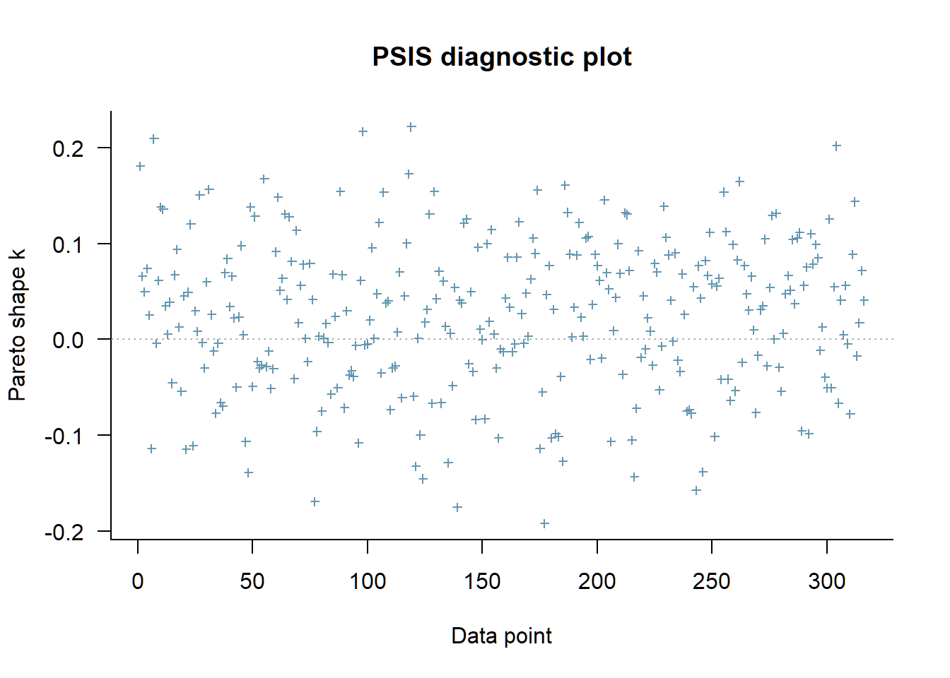
References
This hinted me a missspecification in my testlet models: you can’t estimate a persons skill for a testlet with a single item in it.↩︎
An exception might be the context of adaptive testing where we want to know when our model can predict future responses of a person well enough - or equivalently: when does the incorporation of new responses stop contributing to our model’s predictive precision - so we can stop the measurement.↩︎
Hence we assume the items are conditional independend.↩︎
You can use difficulties or easynesses.↩︎
You might call this abilities or skill values.↩︎
If we integrate out the item parameters as well as the person parameters we’ll get the likelihood used for Bayes factor calculation.↩︎
Nevertheless, the Monte Carlo error for the marginal likelihood is still substantial if your chains ran to short and you have to few posterior samples.↩︎
Rabe-Hesketh et al. (2005) show a spherical approach to efficiently adaptive gaussian quadrature approximation over the latent person variables.↩︎
They calculate the pointwise log-likelihood and then call the corresponding functions in the loo package (Vehtari et al., 2020).↩︎
They substract the fixed effect person covariates from the theta variable - thus their zeta vector should be centered close to zero.↩︎
Although I have to admit that there are some special cases where I don’t find a way to specify all restrictions I want to make for my model within brms syntax (efficiently) and therefore will pass some custom Stan code. One limit I recently found was latent variable modeling as you can do in a SEM but I hope that this feature will come with version 3 - I realy hope you get the founding for the extension of your awesome package, Paul. 😉↩︎
Notice that I used longer chains. To fit the 500 iterations in five chains as described in Merkle et al. (2019) my machine took about 50 seconds.↩︎
If you don’t want to use
::you should userequireinstead oflibraryinside a function.↩︎
Simon Schäfer
Visiting Researcher
My research interests include higher education and Bayesian statistics.